Spike sorting

This utility allows you to perform spike sorting directly from the database, and plot the results.

Link to code

It uses FastICA or PCA followed by HDBSCAN to cluster the spikes.

Note

The current (simple) implementation is mostly meant to help distinguish spikes within the same electrode over a given time period. This is currently not meant to provide an exact “unit” attribution for each spike over longer durations, such as for the lifetime of an organoid on the MEA.
Clusters assignements can and will vary for the same electrode across different time windows, due to the non-deterministic nature of the clustering algorithm.

Introduction

In brief : Choose an electrode and a time window, and the algorithm will return the spikes detected in this window, and their clustering.

Spikes are seperated into two categories :

• Spikes : The spikes detected in the time window. Labels will vary between 0 and \(n_{clusters}\).

  • Outliers : Spikes that were not assigned to any cluster. Those will always be labeled as cluster -1.

• Artifacts : Spikes that were detected as artifacts.
  Those will always be labeled as belonging to cluster -2 to \(-n_{artifacts}\).

  • Artifacts are detected based on their amplitude. If a spike has an amplitude above the artifact_threshold, it will be considered an artifact.

Usage

Creating a SpikeSorting

You may set the following parameters :

• Pre-processing:

  • realign : Whether to realign spikes based on amplitude. Default is True. This is meant to help align spikes that are not perfectly aligned, and have all peaks centered on time 0.

  • time_before : Time before the event to include in the window (in ms). Default is 0.5. Maximum is 1.

  • time_after : Time after the event to include in the window (in ms). Default is 1. Maximum is 2.

    • We recommend keeping the default, as the post-spike noise will cause spurious clustering if the window is too large.

  • artifact_threshold : Threshold to detect artifacts (in uV). Default is 1000. This is meant to detect spikes that are too large to be actual spikes.

  • filter_artifacts : Whether to filter out artifacts. Default is True. If set to False, artifacts will be treated as regular spikes.

• Hyperparameters:

  • dimred_method : Dimensionality reduction method to use. Must be either “PCA” or “ICA”. Default is “PCA”. Recommended to try both.

  • n_components : Number of components to keep after dimensionality reduction. Default is 3. Recommended to try different values.

  • cluster_method : Clustering method to use. Must be either “HDBSCAN” or “OPTICS”. Default is “HDBSCAN”. HDBSCAN is recommended.

  • clustering_kwargs : Additional keyword arguments to pass to the clustering method. Default is None. See the HDBSCAN documentation for more information.

• Miscellaneous:

  • n_jobs : Number of jobs to run in parallel. Default is 8.

    • Avoid setting this too high, as the database will reject too many requests at once.

from dateutil import parser
from datetime import timedelta

from neuroplatform_utils import SpikeSorting

start = parser.parse(
    "2024-10-29 13:00:00"
)  # Change this to the start time of the recording

EXP_NAME = "fs300"
N_COMP = 3
ELECTRODE = 9
sorter = SpikeSorting(dimred_method="ICA", n_components=N_COMP)

Running the SpikeSorting

Hint

See the Database setup page for more information on how to get the experiment ID.

To run the spike sorting, you will need to specify a start and stop time, as well as the experiment ID (fs#ID).

events_df = sorter.run_spike_sorting(
    start, start + timedelta(minutes=20), fs_id=EXP_NAME, electrode_nb=ELECTRODE
)

Plotting the results

Plots reference

The SpikeSorting provides several plots :

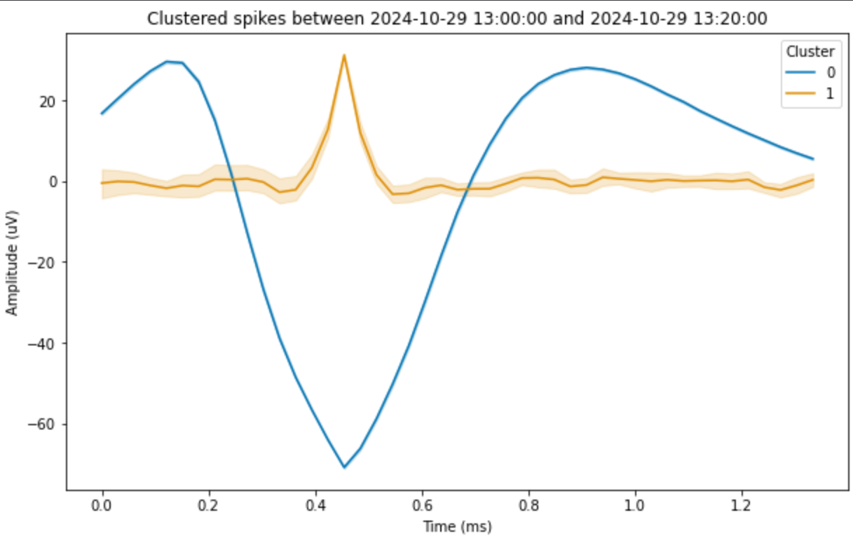
• plot_clustered_spikes : Plot the average waveform of each cluster, with confidence intervals.

  • You may choose to show outliers or not using the show_outliers parameter.

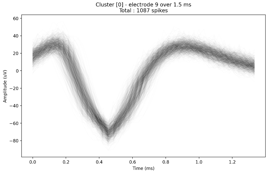
• plot_clustered_artifacts : Plot the average waveform of each artifact cluster, with confidence intervals.

• plot_raw_spikes_for_cluster : Plot all the raw trace of a given cluster.

  • Provide a list of which clusters you wish to see plotted.

• plot_raw_outlier_spikes : Plot all the raw trace of ALL the outliers or artifacts.

  • Provide a list of which clusters you wish to see plotted.

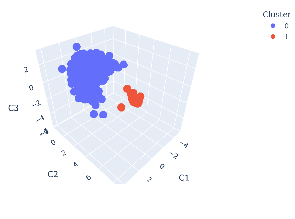
• plot_spike_clustering_in_latent_space : Plot the clustering results in the latent space.

  • This will plot the first 3 components of the dimensionality reduction. If you have more components, the plot may be hard to interpret.

• plot_explained_variance : Plot the explained variance of the PCA. Only available if PCA was used.

Example plots

sorter.plot_clustered_spikes(show_outliers=False)

Fig. 6 Plot of the average waveform of each cluster, with confidence intervals.

sorter.plot_spike_clustering_in_latent_space()

Fig. 7 Plot of the clustering results in the latent space.

sorter.plot_raw_spikes_for_cluster(0)

Fig. 8 Plot of all the raw traces of a given cluster.

Making your own plots

You may also use some of the attributes of the SpikeSorting object to make your own plots :

• raw_spikes_df : DataFrame containing the raw spikes, with clustering results.

• processed_spike_events_df : DataFrame containing the spike events with clustering results.

• dimred_method_spikes.fit_data_df : DataFrame containing the dimensionality reduction, with clustering results.

Hint

Make sure to copy those DataFrames before modifying them, as they are directly linked to the SpikeSorting object.